8  How many monitors are needed in an airshed?

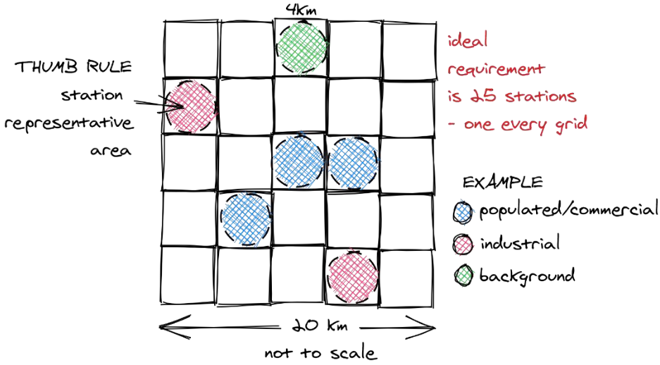
We’ve already learnt in previous tutorials that a single monitor represents only about 10 sq.km of area.

Hence we would need more number of monitors to represent air quality of the entire airshed or a city. In this tutorial, we will learn about CPCB guidelines that estimate the minimum number of monitors needed in an airshed to give a representative value of air quality.

You can also visualise this tool here to find out the number of monitors required in any airshed: Monitoring Needs

8.1 CPCB guidelines

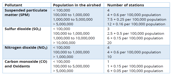
In India, CPCB gave guidelines to determine number of monitors an airshed needs. These guidelines only use population as a factor. Different pollutants would require different number of stations as shown in the picture below:

cpcb_num_monitors_guidelines.png

import numpy as np
def num_monitors_cpcb(pollutant, population):
    if pollutant == 'spm':
        num_station = [4]
        if population < 100000:
            return int(sum(num_station))
        if 1000000 < population:
            num_station.append(np.floor(4 + 0.6*900000/100000)+1)
        else:
            num_station.append(np.floor(4 + 0.6*(population-100000)/100000)+1)

        if 5000000 < population:
            num_station.append(np.floor(7.5 + 0.25*4000000/100000)+1)
        else:
            num_station.append(np.floor(7.5 + 0.25*(population-1000000)/100000)+1)

        if 5000000 < population:
            num_station.append(np.floor(12 + 0.16*(population-5000000)/100000)+1)
            

    if pollutant == 'so2':
        num_station = [3]
        if population < 100000:
            return int(sum(num_station))
        if 1000000 < population:
            num_station.append(np.floor(2.5 + 0.5*900000/100000)+1)
        else:
            num_station.append(np.floor(2.5 + 0.5*(population-100000)/100000)+1)

        if 10000000 < population:
            num_station.append(np.floor(6 + 0.15*9000000/100000)+1)
        else:
            num_station.append(np.floor(6 + 0.15*(population-1000000)/100000)+1)

        if 10000000 < population:
            num_station.append(20)

    if pollutant == 'no2':
        num_station = [4]
        if population < 100000:
            return int(sum(num_station))
        if 1000000 < population:
            num_station.append(np.floor(4 + 0.6*900000/100000)+1)
        else:
            num_station.append(np.floor(4 + 0.6*(population-100000)/100000)+1)

        if 1000000 < population:
            num_station.append(10)

    if pollutant == 'co':
        num_station = [1]
        if population < 100000:
            return int(sum(num_station))
        if 5000000 < population:
            num_station.append(np.floor(1 + 0.15*4900000/100000)+1)
        else:
            num_station.append(np.floor(1 + 0.15*(population-100000)/100000)+1)

        if 5000000 < population:
            num_station.append(np.floor(6 + 0.05*(population-5000000)/100000)+1)

    return int(sum(num_station))
        

num_monitors_cpcb(pollutant='spm',population=5200000)

45

num_monitors_cpcb(pollutant='so2',population=5200000)

24

8.2 Calculating population from Landscan

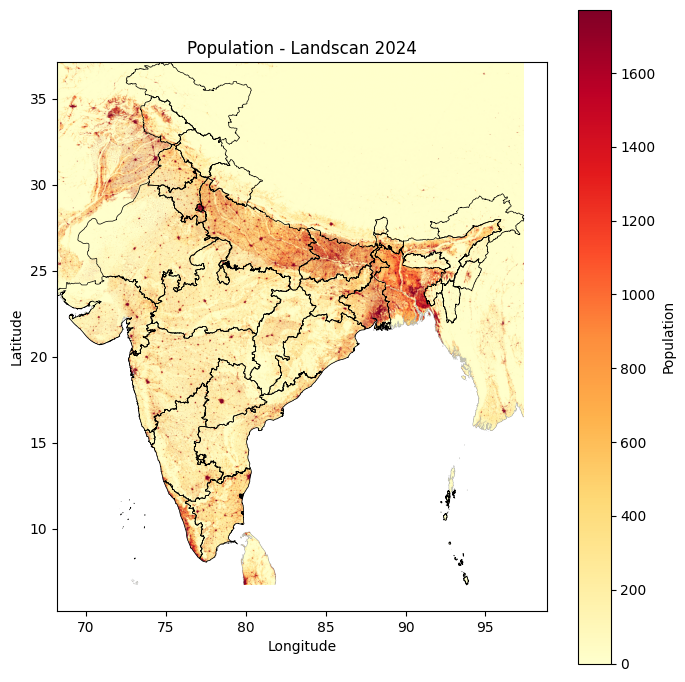
We can dynamically calculate population of any given airshed using the population raster from Landscan. We downloaded the Landscan Global 2024 file, which is a raster image containing population data in ~1km resolution.

import rasterio
import numpy as np
import matplotlib.pyplot as plt
import matplotlib.colors as mcolors
from rasterio.plot import show
import geopandas as gpd

# Load TIFF
tif_path = "data/landscan-india-2024.tif"
with rasterio.open(tif_path) as src:
    population = src.read(1)                        # first band
    population = np.where(population<0, np.nan, population)  # mask nodata encoded as negative
    extent = [src.bounds.left, src.bounds.right, src.bounds.bottom, src.bounds.top]
    crs = src.crs

# Load admin boundaries — reproject to match raster CRS
INDIA_STATES = gpd.read_file('data/INDIA_STATES.geojson').to_crs(crs)
INDIA_STATES.head()

# Plot
fig, ax = plt.subplots(figsize=(7, 7))

im = ax.imshow(
    population,
    extent=extent,
    cmap='YlOrRd',
    origin='upper',
    vmin=np.nanpercentile(population, 2),   # clip outliers
    vmax=np.nanpercentile(population, 98),
)

# Admin boundary overlay
INDIA_STATES.boundary.plot(ax=ax, linewidth=0.5, color='black')

plt.colorbar(im, ax=ax, label='Population')
ax.set_title('Population - Landscan 2024')
ax.set_xlabel('Longitude')
ax.set_ylabel('Latitude')
plt.tight_layout()
#plt.savefig('no2_map.png', dpi=150, bbox_inches='tight')
plt.show()

We can crop this raster to any given airshed. You can download airsheds for India’s NCAP cities from here: Designated Airsheds of 131 India’s NCAP cities | UEInfo. In this tutorial, we work with Mumbai airshed. Mumbai airshed is a big airshed of 6400 sq.km and it also includes Badlapur, Navi Mumbai, Thane, Ulhas Nagar and Vasai Virar.

#Crop the raster to the airshed
from rasterio.mask import mask

tif_path = "data/landscan-india-2024.tif"
with rasterio.open(tif_path) as src:
     #We'll use this for all other rasters 
    target_crs = src.crs
    target_transform = src.transform
    target_width = src.width
    target_height = src.height
    
    mumbai_airshed = gpd.read_file('data/grids_mumbai.kml')
    # Ensure that both Mumbai file and Population raster file has same CRS
    mumbai_airshed = mumbai_airshed.to_crs(src.crs)

    out_image, out_transform = mask(src, mumbai_airshed.geometry, crop=True)
    out_meta = src.meta.copy()

# Update metadata for the new clipped file
out_meta.update({
    "driver": "GTiff",
    "height": out_image.shape[1],
    "width": out_image.shape[2],
    "transform": out_transform
})

#Save the result
with rasterio.open("data/landscan-airshed.tif", "w", **out_meta) as dest:
    dest.write(out_image)

population_airshed = np.where(out_image<0, np.nan, out_image)
print(f'The population of Mumbai airshed is {round(np.nansum(population_airshed)/1000000,2)} Million')

The population of Mumbai airshed is 26.95 Million

We can now send this population value to the num_monitors_cpcb function to calculate number of monitors required as per CPCB to get a representative value of air quality.

num_monitors_cpcb(pollutant='spm',population=np.nansum(population_airshed))

80

Mumbai airshed thus requires a minimum of 80 monitors as per CPCB thumb rule to get representative value of Suspended Partiulate Matter

8.3 Summary

In this tutorial we learnt to use CPCB guidelines to estimate the minimum number of monitors required in an airshed for each pollutant. These guidelines are solely based on the population of the airshed. We thus learnt to calculate the population of the airshed from Landscan rasters and then estimate the monitoring needs.

Note that this estimate is the minimum number of monitors required. In the next tutorial, we will apply urban correction factor to get better estimates.