11  Reading the Air

A tutorial on air quality statistics of a city.

In this tutorial, we will take a monitoring data from a single city (Addis Ababa) and perform basic data analysis required to read the air quality of the city in an informed way.

11.1 Preparing the dataset

This excel file has multiple sheets. Each sheet has houurly data on PM2.5 from each station. The sheet names represent the name of station.

import pandas as pd
import numpy as np
data = pd.read_csv('data/AddisAbaba_hourly_stations_2024.csv')
data.head()
Date pm2.5_a pm2.5_b station Name Lat Long
0 2024-01-01 00:00:00 13.274 15.331 AQN1 AQN1 9.057409 38.763878
1 2024-01-01 01:00:00 14.274 16.330 AQN1 AQN1 9.057409 38.763878
2 2024-01-01 02:00:00 15.459 17.432 AQN1 AQN1 9.057409 38.763878
3 2024-01-01 03:00:00 20.603 23.403 AQN1 AQN1 9.057409 38.763878
4 2024-01-01 04:00:00 33.778 38.040 AQN1 AQN1 9.057409 38.763878
data['pm2.5'] = (data['pm2.5_a'] + data['pm2.5_b'])/2
data['Date'] = pd.to_datetime(data['Date'])
data['year'] = data.Date.dt.year
data['month'] = data.Date.dt.month
data['day'] = data.Date.dt.day
data['hour'] = data.Date.dt.hour
data['day_of_year'] = data.Date.dt.dayofyear
data['DN'] = np.where((data['hour']>=6) & (data['hour']<=20), "D", "N")
data.head()
Date pm2.5_a pm2.5_b station Name Lat Long pm2.5 year month day hour day_of_year DN
0 2024-01-01 00:00:00 13.274 15.331 AQN1 AQN1 9.057409 38.763878 14.3025 2024 1 1 0 1 N
1 2024-01-01 01:00:00 14.274 16.330 AQN1 AQN1 9.057409 38.763878 15.3020 2024 1 1 1 1 N
2 2024-01-01 02:00:00 15.459 17.432 AQN1 AQN1 9.057409 38.763878 16.4455 2024 1 1 2 1 N
3 2024-01-01 03:00:00 20.603 23.403 AQN1 AQN1 9.057409 38.763878 22.0030 2024 1 1 3 1 N
4 2024-01-01 04:00:00 33.778 38.040 AQN1 AQN1 9.057409 38.763878 35.9090 2024 1 1 4 1 N

11.2 City Hourly Statistics

A city’s hourly average PM2.5 is measured as the average of PM2.5 concentrations reported at all stations in the city.

city_hourly = data.groupby(['year','day_of_year','hour'])[['pm2.5']].mean().reset_index()
city_hourly = city_hourly.rename(columns = {'pm2.5':'pm25_avg'})
city_hourly.head()
year day_of_year hour pm25_avg
0 2024 1 0 27.567437
1 2024 1 1 31.128375
2 2024 1 2 35.063125
3 2024 1 3 47.787750
4 2024 1 4 71.411643

Its obvious that at a given hour, different stations report different concentrations. The variation between these concentrations is also an useful measure. Its also useful to know the number of stations used to calculate these statistics.

city_hourly['pm25_std'] = data.groupby(['year','day_of_year','hour'])[['pm2.5']].std().reset_index()['pm2.5']
city_hourly['num_stations'] = data.groupby(['year','day_of_year','hour'])[['pm2.5']].count()['pm2.5'].reset_index()['pm2.5']
city_hourly.head()
year day_of_year hour pm25_avg pm25_std num_stations
0 2024 1 0 27.567437 7.645230 8
1 2024 1 1 31.128375 9.170543 8
2 2024 1 2 35.063125 9.316166 8
3 2024 1 3 47.787750 13.549834 8
4 2024 1 4 71.411643 22.677860 7
Show hidden code that plots city hourly PM2.5 avg
import matplotlib.pyplot as plt
# Create actual datetime
city_hourly['time'] = (
    pd.to_datetime(city_hourly['year'].astype(str), format='%Y')
    + pd.to_timedelta(city_hourly['day_of_year'] - 1, unit='D')
    + pd.to_timedelta(city_hourly['hour'], unit='h')
)

city_hourly = city_hourly.sort_values('time')

# Plot
plt.figure(figsize=(15, 6))

plt.plot(
    city_hourly['time'],
    city_hourly['pm25_avg'],
    label='Mean PM2.5',
    linewidth=1.5
)

plt.fill_between(
    city_hourly['time'],
    city_hourly['pm25_avg'] - city_hourly['pm25_std'],
    city_hourly['pm25_avg'] + city_hourly['pm25_std'],
    alpha=1,
    label='±1 Standard Deviation'
)

plt.xlabel('Time')
plt.ylabel('PM2.5 (µg/m³)')
plt.title('Hourly PM2.5 Variation')
plt.legend()
plt.xticks(rotation=45)
plt.tight_layout()
plt.show()

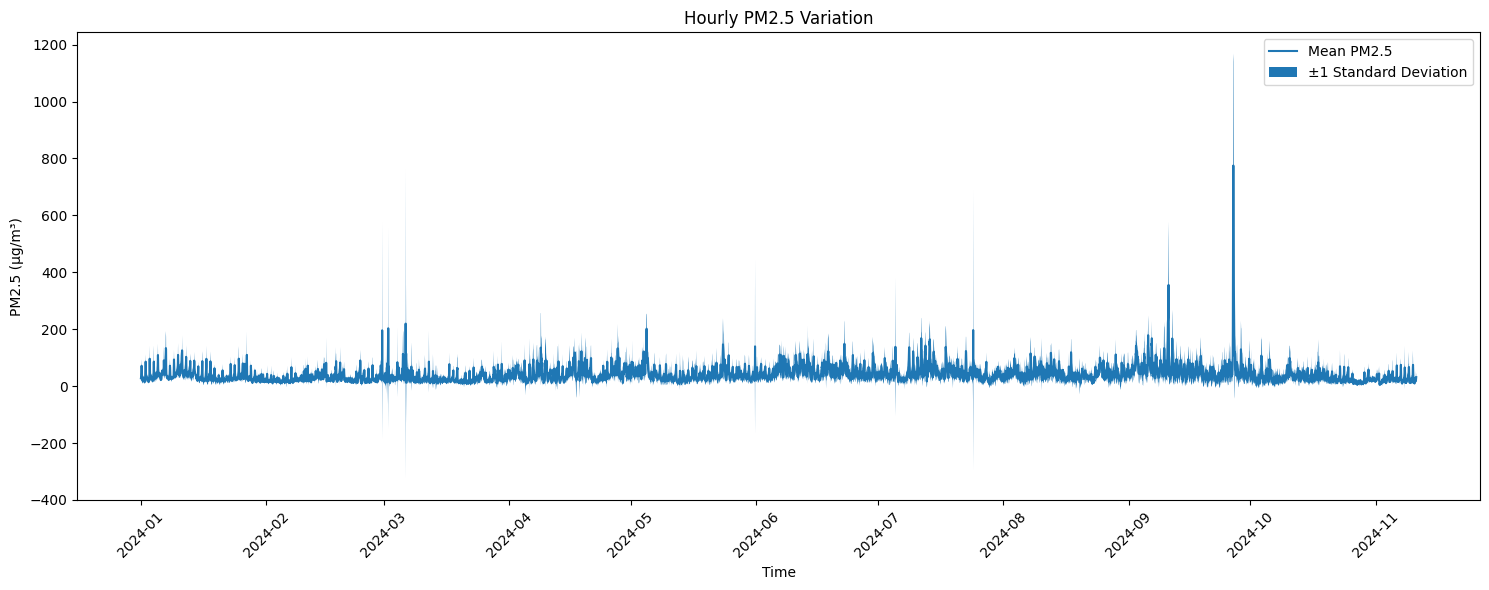
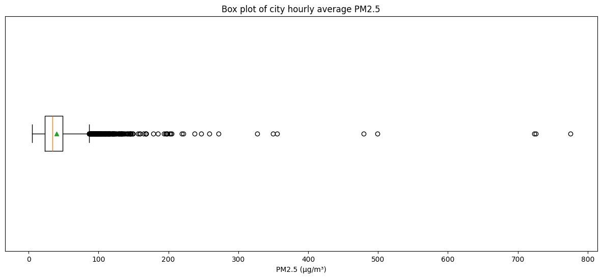
We can see that most hourly averages of the city fall within a narrow range, but there are a few exceptional spikes. We can use percentiles and box-plots to represent them.

# 5 percentile - city hourly average
city_hourly['pm25_avg'].quantile(0.05)
14.274052678571428
# 95 percentile - city hourly average
city_hourly['pm25_avg'].quantile(0.95)
83.66718571428571
plt.figure(figsize=(15, 6))
plt.boxplot(city_hourly['pm25_avg'], vert=False, showmeans=True)
plt.xlabel("PM2.5 (µg/m³)")
plt.yticks([],[])
plt.title("Box plot of city hourly average PM2.5")
plt.show()

11.3 City Daily Statistics

When we have station hourly data, it is better to use that to calculate city daily statistics. If we use city hourly averages to calculate daily average, each hour’s average gets equally weighted. But we know that if an hour’s average is calculated from more number of stations, it is better. Hence, City average PM2.5 concentration on any day is the average of all station hourly values on that day.

city_daily = data.groupby(['year','day_of_year'])['pm2.5'].agg(['mean','std','count']).reset_index()
city_daily.head()
year day_of_year mean std count
0 2024 1 27.148908 16.185248 190
1 2024 2 30.879924 19.781855 171
2 2024 3 35.244666 22.693411 148
3 2024 4 38.370046 21.220646 184
4 2024 5 43.599324 24.039891 196
Show hidden code that plots city daily PM2.5 avg
# Create actual datetime
city_daily['time'] = (
    pd.to_datetime(city_daily['year'].astype(str), format='%Y')
    + pd.to_timedelta(city_daily['day_of_year'] - 1, unit='D')
)

city_daily = city_daily.sort_values('time')

# Plot
plt.figure(figsize=(15, 6))

plt.plot(
    city_daily['time'],
    city_daily['mean'],
    label='Mean PM2.5',
    linewidth=1.5
)

plt.fill_between(
    city_daily['time'],
    city_daily['mean'] - city_daily['std'],
    city_daily['mean'] + city_daily['std'],
    alpha=0.3,
    label='±1 Standard Deviation'
)

plt.xlabel('Time')
plt.ylabel('PM2.5 (µg/m³)')
plt.title('Daily PM2.5 Variation')
plt.axhline(15, color='darkgreen', linestyle='--', label='W.H.O Daily PM2.5 Target')
plt.legend()
plt.xticks(rotation=45)
plt.tight_layout()
plt.show()

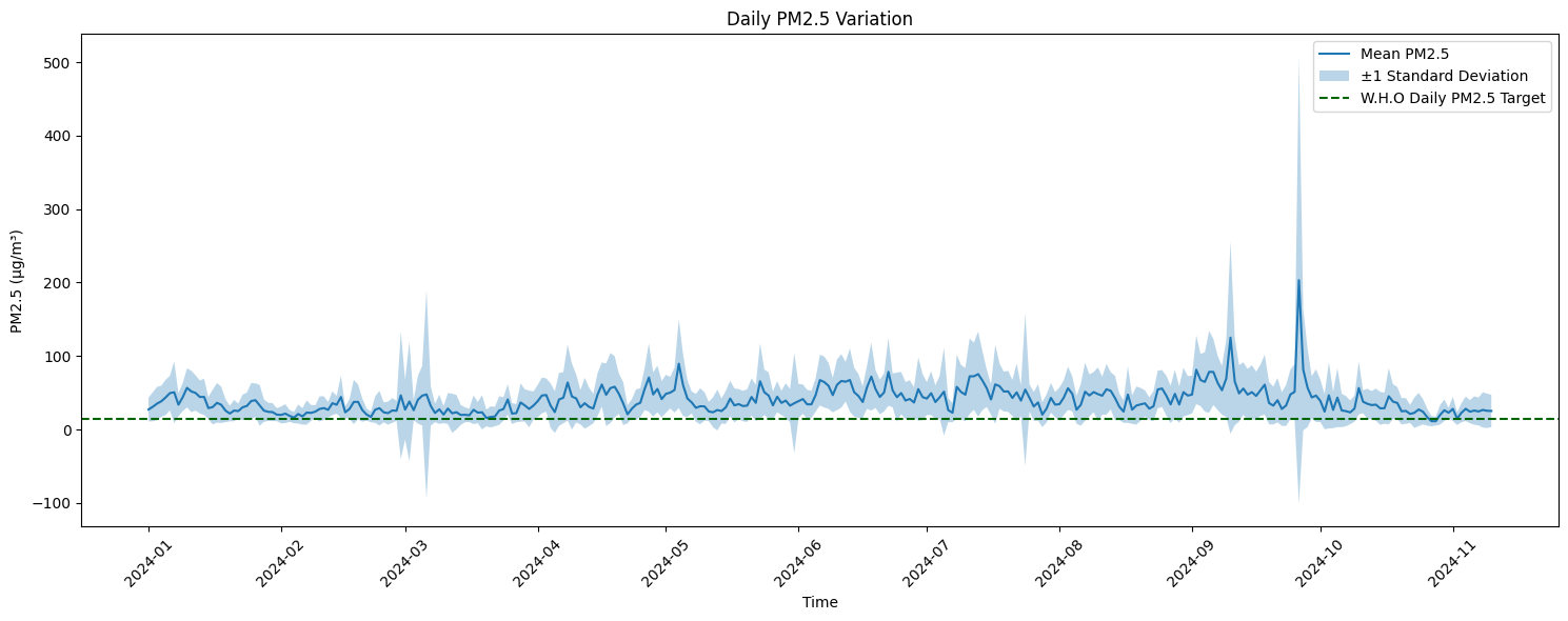
We can apply W.H.O’s Air Quality Standards at daily statistics. W.H.O recommended a daily average level of 15 µg/m³ for PM2.5 As per W.H.O, a city should meet these daily averages on 99% of the days. We can see that Addis Ababa meets this target in less than 1% of days.

(city_daily['mean']<15).mean()*100
0.9523809523809524
# 5 percentile - city hourly average
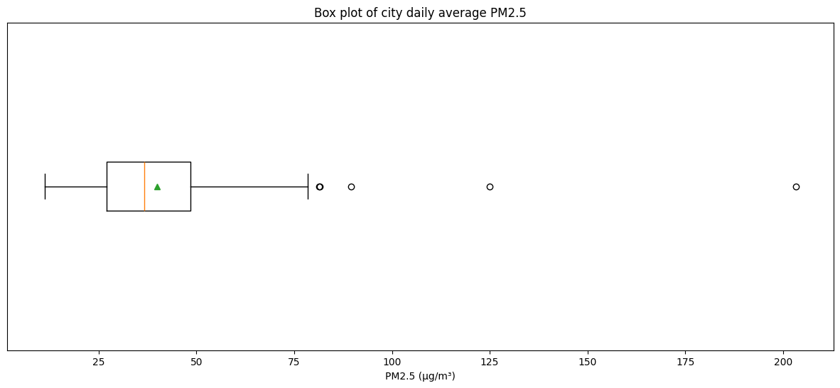
city_daily['mean'].quantile(0.05)
20.070973771880293
# 95 percentile - city hourly average
city_daily['mean'].quantile(0.95)
67.27227463787735
plt.figure(figsize=(15, 6))
plt.boxplot(city_daily['mean'], vert=False, showmeans=True)
plt.xlabel("PM2.5 (µg/m³)")
plt.yticks([],[])
plt.title("Box plot of city daily average PM2.5")
plt.show()

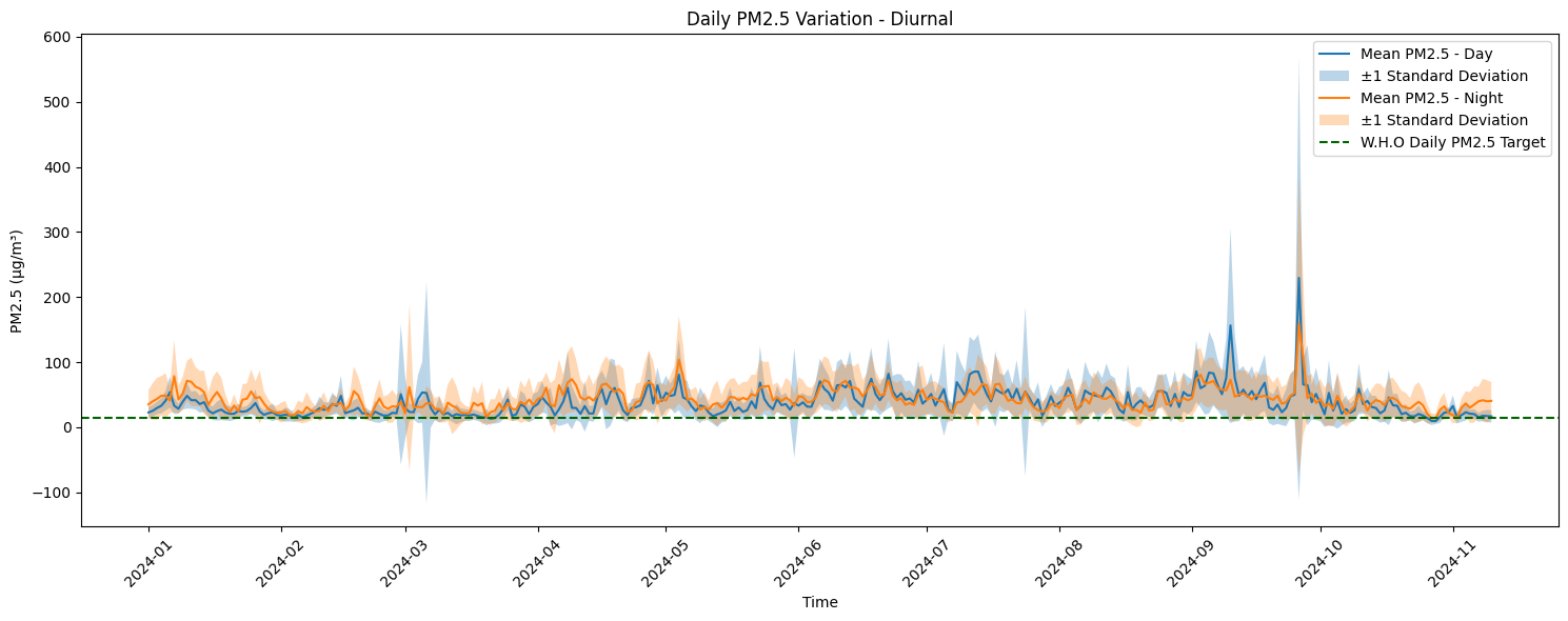
Within a day, we can also start making diurnal analysis - comparing day and night

city_daily_diurnal = data.groupby(['year','day_of_year','DN'])['pm2.5'].agg(['mean','std','count']).reset_index()
city_daily_diurnal.head()
year day_of_year DN mean std count
0 2024 1 D 22.675828 8.755595 122
1 2024 1 N 35.174140 22.332102 68
2 2024 2 D 25.366575 8.803188 106
3 2024 2 N 39.870923 27.925978 65
4 2024 3 D 29.655708 9.548785 89
Show hidden code that plots city daily PM2.5 avg - diurnal
# Create actual datetime
city_daily_diurnal['time'] = (
    pd.to_datetime(city_daily_diurnal['year'].astype(str), format='%Y')
    + pd.to_timedelta(city_daily_diurnal['day_of_year'] - 1, unit='D')
)

city_daily_diurnal = city_daily_diurnal.sort_values('time')

# Plot
plt.figure(figsize=(15, 6))

city_daily_day = city_daily_diurnal[city_daily_diurnal['DN']=='D']
plt.plot(
    city_daily_day['time'],
    city_daily_day['mean'],
    label='Mean PM2.5 - Day',
    linewidth=1.5
)

plt.fill_between(
    city_daily_day['time'],
    city_daily_day['mean'] - city_daily_day['std'],
    city_daily_day['mean'] + city_daily_day['std'],
    alpha=0.3,
    label='±1 Standard Deviation'
)


city_daily_night = city_daily_diurnal[city_daily_diurnal['DN']=='N']
plt.plot(
    city_daily_night['time'],
    city_daily_night['mean'],
    label='Mean PM2.5 - Night',
    linewidth=1.5
)

plt.fill_between(
    city_daily_night['time'],
    city_daily_night['mean'] - city_daily_night['std'],
    city_daily_night['mean'] + city_daily_night['std'],
    alpha=0.3,
    label='±1 Standard Deviation'
)

plt.xlabel('Time')
plt.ylabel('PM2.5 (µg/m³)')
plt.title('Daily PM2.5 Variation - Diurnal')
plt.axhline(15, color='darkgreen', linestyle='--', label='W.H.O Daily PM2.5 Target')
plt.legend()
plt.xticks(rotation=45)
plt.tight_layout()
plt.show()

11.4 City Monthly Statistics

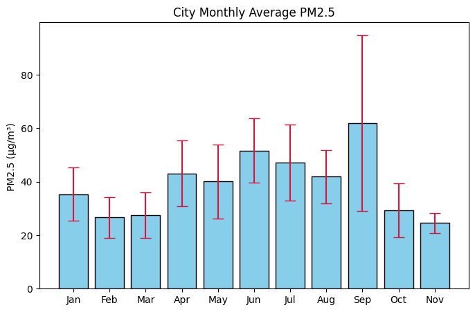
We’ll now use the city daily averages data to produce monthly and seasonal statistics. We are thus assuming that each day’s average is equally valid as cities report daily averages officially.

city_daily['month'] = city_daily.time.dt.strftime('%b')
city_daily.head()
year day_of_year mean std count time month
0 2024 1 27.148908 16.185248 190 2024-01-01 Jan
1 2024 2 30.879924 19.781855 171 2024-01-02 Jan
2 2024 3 35.244666 22.693411 148 2024-01-03 Jan
3 2024 4 38.370046 21.220646 184 2024-01-04 Jan
4 2024 5 43.599324 24.039891 196 2024-01-05 Jan
import calendar
month_order = list(calendar.month_abbr)[1:]
city_daily['month'] = pd.Categorical(city_daily['month'], categories=month_order, ordered=True)

city_monthly = city_daily.groupby(['year','month'])['mean'].agg(['mean','std']).reset_index().dropna()
city_monthly.head()
/tmp/ipykernel_4307/594153622.py:5: FutureWarning: The default of observed=False is deprecated and will be changed to True in a future version of pandas. Pass observed=False to retain current behavior or observed=True to adopt the future default and silence this warning.
  city_monthly = city_daily.groupby(['year','month'])['mean'].agg(['mean','std']).reset_index().dropna()
year month mean std
0 2024 Jan 35.302709 9.964558
1 2024 Feb 26.600191 7.697346
2 2024 Mar 27.499748 8.425786
3 2024 Apr 43.046578 12.247179
4 2024 May 40.049051 13.820356
fig, ax = plt.subplots(figsize=(8,5))
ax.bar(city_monthly['month'], city_monthly['mean'], yerr=city_monthly['std'].to_numpy(),
       color='skyblue', edgecolor='black', capsize=6, ecolor='crimson')
plt.title('City Monthly Average PM2.5')
plt.ylabel('PM2.5 (µg/m³) ')
plt.show()

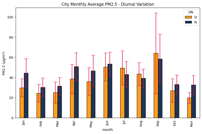
Diurnal

# Create actual datetime
city_daily_diurnal['time'] = (
    pd.to_datetime(city_daily_diurnal['year'].astype(str), format='%Y')
    + pd.to_timedelta(city_daily_diurnal['day_of_year'] - 1, unit='D')
)

city_daily_diurnal['month'] = city_daily_diurnal.time.dt.strftime('%b')

month_order = list(calendar.month_abbr)[1:]
city_daily_diurnal['month'] = pd.Categorical(city_daily_diurnal['month'], categories=month_order, ordered=True)

city_monthly_diurnal = city_daily_diurnal.groupby(['year','month','DN'])['mean'].agg(['mean','std']).reset_index().dropna()
city_monthly_diurnal.head()
/tmp/ipykernel_4307/1780426900.py:12: FutureWarning: The default of observed=False is deprecated and will be changed to True in a future version of pandas. Pass observed=False to retain current behavior or observed=True to adopt the future default and silence this warning.
  city_monthly_diurnal = city_daily_diurnal.groupby(['year','month','DN'])['mean'].agg(['mean','std']).reset_index().dropna()
year month DN mean std
0 2024 Jan D 29.774738 9.088560
1 2024 Jan N 44.548786 14.189184
2 2024 Feb D 24.306320 8.680840
3 2024 Feb N 30.272460 9.156744
4 2024 Mar D 25.078230 10.689991
df_mean = city_monthly_diurnal.pivot(index='month', columns='DN', values='mean')
df_std = city_monthly_diurnal.pivot(index='month', columns='DN', values='std')

fig, ax = plt.subplots(figsize=(10,6))
df_mean.plot(kind='bar', yerr=df_std, ax=ax, color=["#FF9F1C","#1D3557"],edgecolor='black', capsize=6, ecolor='crimson')
plt.title('City Monthly Average PM2.5 - Diurnal Variation')
plt.ylabel('PM2.5 (µg/m³) ')
plt.show()

11.5 City Annual Statistics

The W.H.O’s Annual Standard for PM2.5 is 5 µg/m³. Addis Ababa is thus 8 times more than W.H.O standard.

#Annual average
city_daily.groupby(['year'])[['mean']].agg(['mean','std'])
mean
mean std
year
2024 39.899716 17.998168
city_daily_diurnal.groupby(['year','DN'])[['mean']].agg(['mean','std'])
mean
mean std
year DN
2024 D 38.157480 21.017833
N 42.718817 16.108997

11.6 Spatial Heterogeniety

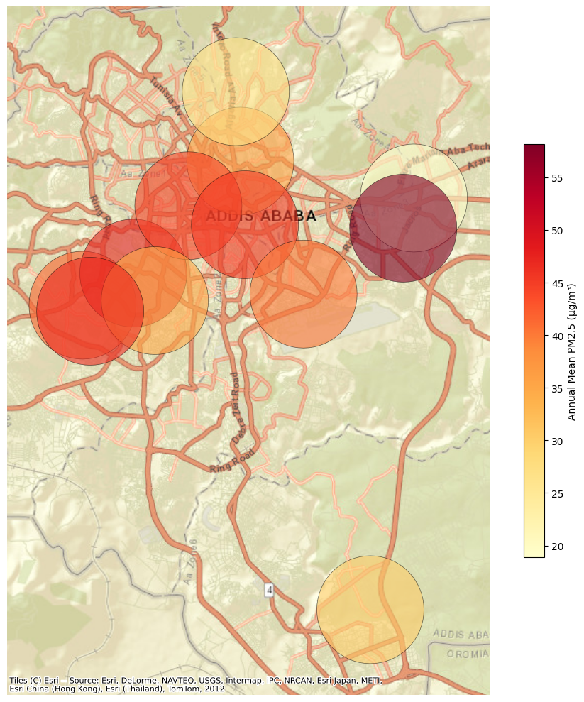
We can see spatial heterogeneity in the pollutoin by visualising station level stats. Let’s plot station level annual means.

station_daily = data.groupby(['year','station','day_of_year'])['pm2.5'].agg(['mean','std','count']).reset_index()
station_annual = station_daily.groupby(['year','station'])['mean'].agg(['mean']).reset_index()
station_annual = station_annual.merge(data[['station','Lat','Long']]).drop_duplicates().reset_index(drop=True)

station_annual
year station mean Lat Long
0 2024 AAEPGDC 18.893042 9.021745 38.824353
1 2024 AASTUMAIA 30.296063 8.883660 38.809601
2 2024 AAU4K 36.025417 9.034121 38.765430
3 2024 AHRI 41.562116 8.985801 38.711855
4 2024 AQ10_ICSL 47.461347 8.996560 38.729099
5 2024 AQN1 27.084370 9.057409 38.763878
6 2024 AQN2 58.164605 9.011622 38.820760
7 2024 BLH 44.542067 9.019170 38.747780
8 2024 ECA 45.331427 9.012812 38.767014
9 2024 PCO 35.144690 8.987340 38.736390
10 2024 REPPIE 46.753306 8.983766 38.714447
11 2024 Skyline 40.344499 8.989531 38.786888
Show hidden code that plots monitors locations along with Annual Mean PM2.5 values.
import geopandas as gpd
import contextily as cx
import matplotlib.pyplot as plt

# df has: station, lat, long, mean
gdf = gpd.GeoDataFrame(
    station_annual,
    geometry=gpd.points_from_xy(station_annual["Long"], station_annual["Lat"]),
    crs="EPSG:4326",
)

# Buffer in a local metric CRS (UTM) so 2000 m is accurate,
# then reproject to Web Mercator for the basemap
utm = gdf.estimate_utm_crs()
circles = gdf.to_crs(utm).copy()
circles["geometry"] = circles.geometry.buffer(2000)   # 2 km radius
circles = circles.to_crs(epsg=3857)

fig, ax = plt.subplots(figsize=(10, 10))
circles.plot(
    column="mean",
    cmap="YlOrRd",
    alpha=0.6,
    edgecolor="black",
    linewidth=0.5,
    legend=True,
    legend_kwds={"label": "Annual Mean PM2.5 (µg/m³)", "shrink": 0.6},
    ax=ax,
)

cx.add_basemap(ax, source=cx.providers.Esri.WorldStreetMap)   # no key
ax.set_axis_off()
plt.tight_layout()
plt.show()

Each station represents a circular area of about 2km radius. We can thus see that the monitor network is not well distributed.