6  Source Apportionment

In the previous tutorials, we learnt to answer the following questions:

1. How much is the pollution?
2. Where is the pollution? and
3. When is the pollution?

But it is also important that we know the sources of the pollution in a city. Only by knowing sources that we can think of reducing ways to reduce pollution. We know about sources of pollution by conducting source apportionment studies.

The source apportionment studies are not easy to conduct. They require a lot of skilled personnel for monitoring, data modeling, laboratory facilities and financial support. There are a few institutions that have the wherewithal to conduct source apportionment studies. There are two ways in which source apportionment can be done:

1. Top-down way: Using Receptor Modeling (RM)

2. Bottom-up way: Emissions Modeling.

What is Source Apportionment? A Primer by UrbanEmissions.Info

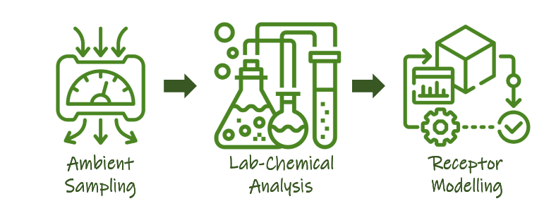
6.1 Top-down: Receptor Modeling (RM) based source apportionment

SA_topdown.png

The World Health Organisation (W.H.O) collected source apportionment studies performed in various cities across the world between 1990-2014. This is a good dataset to explore source apportionment.

Database on source apportionment studies for particulate matter - W.H.O

import pandas as pd
who_sources_db = pd.read_csv('data/database_source_apport_studies_v2_0_26_9_2015.csv')
who_sources_db.sample(5)

	Site Location	Population estimate *	Country	ISO 3 code	Country Region	continent	Latitude	Longitude	Site typology	PM10 µgm-3 *	...	Reference author	Reference year	Study year	Season	SEA SALT%	DUST%	TRAFFIC%	INDUSTRY%	BIOM. BURN./RES.%	OTHER (unspecified-human origin)%
293	Santander	1,78,475	Spain	ESP	Southwestern Europe	EU	43.47	-3.81	urban	NaN	...	Moreno171,172	2011.0	2007/8	year	13.0	1.0	37.0	7.0	NaN	42.0
503	Rio de Janeiro	63,20,000	Brazil	BRA	Brazil	SA	-22.90	-43.21	urban	NaN	...	Godoy5	2009.0	2003/2005	year	NaN	36.0	29.0	35.0	NaN	0.0
439	Corpus Christi	3,12,195	USA	USA	USA	NaN	27.42	-97.29	rural	NaN	...	Subramoney116	2013.0	2003/2005	year	15.0	4.0	26.0	NaN	3.0	52.0
270	La Linea	64,645	Spain	ESP	Southwestern Europe	EU	36.16	-5.35	urban-industrial	NaN	...	Amato128–131	2014.0	2003/2010	year	9.0	5.0	25.0	14.0	NaN	47.0
492	Jamari(†)	< 50	Brazil	BRA	Brazil	SA	-9.20	-63.17	rural	105.0	...	Artaxo2,3	1998.0	1995	fall	5.9	21.3	NaN	NaN	54.0	18.8

5 rows × 22 columns

SEA SALT, DUST, TRAFFIC, INDUSTRY, BIOMASS BURNING/RESIDENTIAL and OTHERS are the sources recognised in this database for each city.

sources = ['SEA SALT%', 'DUST%', 'TRAFFIC%', 'INDUSTRY%', 'BIOM. BURN./RES.%',
       'OTHER (unspecified-human origin)%']

The W.H.O database is a collection of all RM source apportionment studies. We can see that there are several methods of performing an RM study.

who_sources_db['Methodology'].unique()

array(['PCA', 'CMB', 'PMF', 'UNMIX', 'APCS', 'FA', 'LENSCHOW', 'ME',
       'PCA-MLR', 'PCA/APCS', 'CMF', 'COPREM', 'APEG', 'PCFA', 'APCFA',
       'MC', 'PMF-ME', 'PMF-UNMIX', 'CMB/UNMIX', 'APCA', 'APFA', nan],
      dtype=object)

6.1.1 Source apportionment pie

Let’s learn to build a source apportionment pie for the city Beijing using the 2010 study.

required_columns  = ['Site Location','Country','Site typology', 'PM2.5 µgm-3 *', 'Methodology', 'Season']+sources
city = 'Beijing'
year = '2010'

Beijing_2010_SA = who_sources_db[(who_sources_db['Site Location']==city)&(who_sources_db['Study year']==year)][required_columns]
Beijing_2010_SA

	Site Location	Country	Site typology	PM2.5 µgm-3 *	Methodology	Season	SEA SALT%	DUST%	TRAFFIC%	INDUSTRY%	BIOM. BURN./RES.%	OTHER (unspecified-human origin)%
98	Beijing	China	urban	55	PMF	year	NaN	10.4	29.7	22.0	11.2	26.7

From this source apportionment study, we can infer the following details:

1. The annual PM2.5 concentration in Beijing in 2010 was 55 µg/m3.
2. The source apportionment study was performed by the PMF method (Positive Matrix Factorization). It is a Receptor Modeling (RM) method. You can read more about it here: Positive Matrix Factorization Model for Environmental Data Analyses | US EPA
3. TRAFFIC is the major source of PM2.5 followed byINDUSTRY, BIOMASS BURNING/RESIDENTIAL and DUST.

import matplotlib.pyplot as plt
source_contributions = list(Beijing_2010_SA[sources].dropna(axis=1).values.flatten())
sources = Beijing_2010_SA[sources].dropna(axis=1).columns

fig, ax = plt.subplots()
ax.pie(source_contributions,
       labels=sources,
       autopct='%1.1f%%')
plt.show()

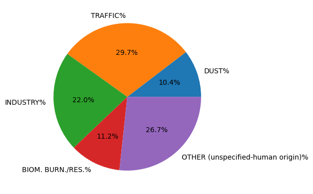
We can also calculate the contributions of each source to PM2.5 in µg/m3 by multiplying the total PM2.5 concentration with source percentage.

pm25 = float(Beijing_2010_SA['PM2.5 µgm-3 *'].values[0])

print(f"Beijing's annual PM2.5 concentration in 2010 is {pm25} µg/m3 \n Of which, the contribution of:")
for source, contribution in zip(sources,source_contributions):
    print(f"{source[:-1]} is {round(contribution*pm25/100,2)} µg/m3")

Beijing's annual PM2.5 concentration in 2010 is 55.0 µg/m3 
 Of which, the contribution of:
DUST is 5.72 µg/m3
TRAFFIC is 16.34 µg/m3
INDUSTRY is 12.1 µg/m3
BIOM. BURN./RES. is 6.16 µg/m3
OTHER (unspecified-human origin) is 14.68 µg/m3

We know that W.H.O annual standard of PM2.5 is 5 µg/m3. Thus, the least contributive source DUST alone was responsible in Beijing to cross the W.H.O standard. This gives us some insight on where to focus in reducing pollution.

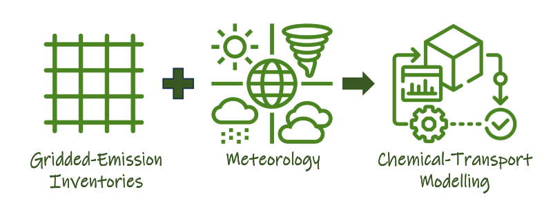
6.2 Bottom-up: Emissions based Source Apportionment

SA_bottomup.png

Another way to estimate source contributions is from sector specific emissions in a city. The advantage of using Emissions based approach is that we can forecast emissions of a city and thus forecast future sources of air pollution.

UrbanEmissions.Info performed emissions based PM2.5 source apportionment studies for various cities in India as part of the Air Pollution Knowledge Assessment (APnA) City Program. You can see the source apportionment pies of these cities, here: Link

apna = pd.read_csv('data/APnA_50airsheds_PM25_Source_Apportionment_CAMxOutputs.csv')
apna.tail()

	Airshed	City	Transport	Residential	Industrial	Dust	Waste	Diesel Genset	Brick Kiln	Sea Salt	External	study_year
44	45	Nagpur	17.20%	6.80%	26.70%	10.90%	11.60%	1.80%	3.20%	NaN	21.40%	2017
45	46	Patna	14.80%	14.60%	11.20%	12.10%	12.90%	5.40%	9.30%	NaN	19.20%	2017
46	47	Pune-Pimpri-Chinchwad	24.00%	5.80%	9.80%	23.40%	6.40%	2.80%	2.60%	NaN	24.70%	2017
47	48	Raipur-Durg-Bhillai	17.20%	11.80%	22.80%	11.50%	6.20%	2.80%	1.40%	NaN	25.80%	2017
48	49	Ranchi	21.10%	18.00%	1.10%	14.10%	12.20%	1.30%	3.20%	NaN	28.50%	2017

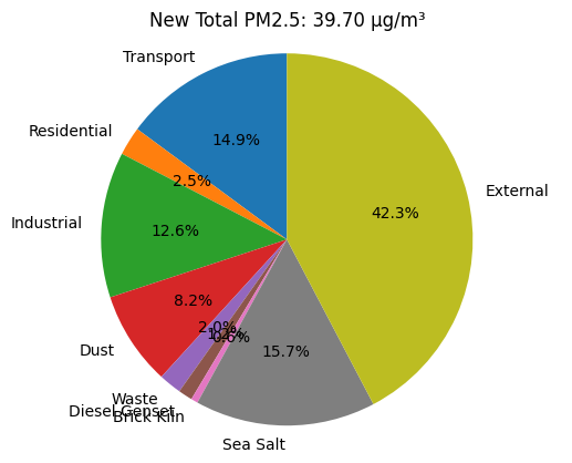
We can note that this study identified more sources than the previous one: Transport, Residential, Dust, Waste, Diesel Genset, Brick Kiln, Sea Salt and External.

sources =  ['Transport', 'Residential', 'Industrial', 'Dust', 'Waste', 'Diesel Genset', 'Brick Kiln', 'Sea Salt', 'External']

6.2.1 Scenario building

When we have source apportionment data, we can also build various scenarios of air pollution. We will build a scenario for the city of Mumbai. You can download the APnA leaflet for Mumbai from here: Mumbai APnA 2019.

In 2018, the annual average PM2.5 concentration in Mumbai was 51.5 µg/m3. We can obtain source contributions from the APnA dataset.

pm25_mumbai = 51.5 #µg/m3
mumbai_sources = apna[apna.City =='Mumbai']
mumbai_sources

	Airshed	City	Transport	Residential	Industrial	Dust	Waste	Diesel Genset	Brick Kiln	Sea Salt	External	study_year
17	18	Mumbai	16.40%	3.20%	15.00%	12.60%	3.80%	1.90%	2.30%	12.10%	32.60%	2019

# Percentage reduction in each source
reductions={'Transport':30,'Residential':40, 'Industrial':35, 'Dust':50, 'Waste':60, 'Diesel Genset':50,
            'Brick Kiln':80, 'Sea Salt':0, 'External':0}

import ipywidgets as widgets
from IPython.display import display

# Source contributions in #µg/m3
base_contrib = mumbai_sources[sources].T
base_contrib.columns = ['source_contribution']
base_contrib = base_contrib.source_contribution.str[:-1].astype(float)*pm25_mumbai/100
pm25_mumbai_ = round(base_contrib.sum(),2)


sliders = {}

for col in sources:
    sliders[col] = widgets.FloatSlider(
        value=reductions[col], min=0, max=100, step=1,
        description=col,
        continuous_update=False
    )

def update(**reductions):
    new_contrib = base_contrib.copy()
    
    for source, reduction in reductions.items():
        new_contrib[source] *= (1 - reduction/100)

    new_total = round(new_contrib.sum(),2)
    
    # ---- PIE CHART ----
    plt.figure()
    
    # # optional: remove very small slices for clarity
    # plot_data = new_contrib[new_contrib > 2]
    
    plt.pie(
        new_contrib,
        labels=new_contrib.index,
        autopct='%1.1f%%',
        startangle=90
    )
    
    plt.title(f"New Total PM2.5: {new_total:.2f} µg/m³")
    plt.axis('equal')  # keeps it circular
    
    plt.show()
    
    print(f"Original: {pm25_mumbai_:.2f} µg/m³")
    print(f"New: {new_total:.2f} µg/m³")
    print(f"Reduction: {pm25_mumbai_ - new_total} µg/m³")
    
update(**{k:reductions[k] for k in sliders})

Original: 51.45 µg/m³
New: 39.70 µg/m³
Reduction: 11.75 µg/m³

ui = widgets.VBox(list(sliders.values()))
out = widgets.interactive_output(update, sliders)
title = widgets.HTML("<h3>Adjust Source Reductions (%)</h3>")
display(title, ui, out)

We can thus play with various scenarios and see when the city of Mumbai can meet the Air Quality Standards. The above is one such scenario when we can observe that Mumbai’s PM2.5 annual average met NAAQS of 40µg/m³. Ofcourse, if the specified reductions are practical or not is another debate. But with these scenario players we can start thinking about solutions to the air pollution problem

6.3 Summary

In this tutorial, we learnt what is source apportionment and various methods of performing source apportionment studies. We explored the database on source apportionment studies and worked with Beijing’s data to create a source apportionment pie. We then built a scenario player using Mumbai’s emission based source apportionment study and saw how Mumbai can reach NAAQS standard of 40 µg/m³.